Analyzer Optimizations¶

The original implementation of Skyline has worked for years, almost flawlessly it must be said. However the original implementation of Skyline was patterned and somewhat even hard coded to run in a very large and powerful setup in terms of the volume of metrics it was handling and the server specs it was running on.

This setup worked and ran OK on all metric volumes. However if Skyline was setup in a smaller environment with a few 1000 metrics, the CPU graphs and load_avg stats of your Skyline server suggested that Skyline did need a LOT of processing power. However this is no longer true.

This was due to one single line of code at the end of Analyzer module, which only slept if the runtime of an analysis was less than 5 seconds, undoubtedly resulted in a lot of Skyline implementations seeing constantly high CPU usage and load_avg when running Skyline. As this resulted in Analyzer running in say 19 seconds and then immediately spawning again and again, etc.

https://github.com/etsy/skyline/blob/master/src/analyzer/analyzer.py#L242

# Sleep if it went too fast
if time() - now < 5:
    logger.info('sleeping due to low run time...')
    sleep(10)

Number of Analyzer processors¶

A number of optimizations have changed the required number of processors to assign to settings.ANALYZER_PROCESSES, quite dramatically in some cases. Specifically in cases where the number of metrics being analyzed is not in the 10s of 1000s.

Python multiprocessing is not very efficient if it is not need, in fact the overall overhead of the spawned processes ends up greater than the overhead of processing with a single process. For example, if we have a few 1000 metrics and we have 4 processors assigned to Analyzer and the process duration is 19 seconds, in the original Analyzer we would have seen 4 CPUs running at 100% constantly (due to the above Sleep if it went to fast). Even if we leave to Sleep if went too fast in and we change to settings.ANALYZER_PROCESSES to 1, we will find that:

1. we now see 1 CPU running at 100%
1. our duration has probably increased to about 27 seconds
1. we use a little more memory on the single process

When we optimize the sleep to match the environment with the settings.ANALYZER_OPTIMUM_RUN_DURATION of in this case say 60 instead of 5, we will find that:

1. we now see 1 CPU running at a few percent, only spiking up for 27 seconds

When we further optimize and use the settings.RUN_OPTIMIZED_WORKFLOW we will find that:

1. we now see 1 CPU running at a few percent, only spiking up for 14 seconds
1. our duration has probably decreased to about 50%

See Optimizations results at the end of this page.

Analyzer work rate¶

The original Analyzer analyzed all timeseries against all algorithms which is the maximum possible work. In terms of the settings.CONSENSUS based model, this is not the most efficient work rate.

Performance tuning¶

A special thanks to Snakeviz for a very useful Python profiling tool which enabled some minimal changes in the code and substantial improvements in the performance, along with cprofilev and vmprof.

Using anomaly_breakdown metrics graphs to tune the Analyzer workflow¶

anomaly_breakdown metrics were added to Skyline on 10 Jun 2014, yet never merged into the main Etsy fork. However, in terms of performance tuning and profiling Skyline they are quite useful. They provide us with the ability to optimize the analysis of timeseries data based on 2 simple criteria:

Determine the algorithms that are triggered most frequently
Determine the computational expense of each algorithm (a development addition) that adds algorithm_breakdown.*.timing.times_run and the algorithm_breakdown.*.timing.total_time metrics to skyline.analyzer. hostname graphite metric namespaces.

We can use these data to determine the efficiency of the algorithms and when this is applied to the Analyzer settings.CONSENSUS model we can optimize algorithms.py to run in the most efficient manner possible.

Originally algorithms.py simply analyzed every timeseries against every algorithm in ALGORITHMS and only checked the settings.CONSENSUS threshold at the end. However a very small but effective optimization is to use the above data to run the following optimizations.

The most frequently and least expensive settings.CONSENSUS number of algorithms and then determine if settings.CONSENSUS can be achieved. Currently there are 9 algorithms that Analyzer uses. However the same optimization is valid if more algorithms were added.
If our settings.CONSENSUS was 6 and Analyzer has not been able to trigger any of the most frequently and least expensive 5 algorithms, then there is no need to analyze the timeseries against the remaining algorithms. This surprisingly reduces the work of Analyzer by ~xx% on average (a lot).
The cost of this optimization is that we lose the original algorithm_breakdown.* metrics which this was evaluated and patterned against. However two additional factors somewhat mitigate this but it is definitely still skewed. The mitigations being that:
- When a timeseries is anomalous more than one algorithm triggers anyway.
- When an algorithm is triggered, more algorithms are run. Seeing as we have optimized to have the least frequently triggered algorithms be run later in the workflow, it stands to reason that a lot of the time, they would not have triggered even if they were run. However it is still skewed.

These optimizations are now the default in settings.py, however they have been implemented with backwards compatibility and for the purpose of running Analyzer without optimization of the algorithms to ensure that they can be benchmarked again should any further algorithms ever be added to Analyzer or any existing algorithms modified in any way.

algorithm benchmarks¶

analyzer_dev can be/was used as a benchmarking module to determine the execution times of algorithms.

Considerations - approximation of timings¶

The algorithm benchmark timings are simply approximations of the real times that the algorithm execution is undertaken in (float).

tmpfs vs multiprocessing Value¶

Recording the algorithm counts and timings without using multiprocessing Value and associated overhead of locks, etc, etc. /tmp was opted for instead and the variable settings.SKYLINE_TMP_DIR was added. In most cases /tmp is tmpfs which is memory anyway so all the heavy lifting in terms of locking etc is offloaded to the OS and modules do not have to incur the additional complexity in Python. A simple yet effective win. Same same but different. There may be some valid reasons for the use multiprocessing Value or Manager().list()

Algorithms ranked by triggered count¶

Using the anomaly_breakdown metrics data it shows that on a plethora of machine and application related metrics, we can determine the most triggered algorithms by rank:

stddev_from_average
mean_subtraction_cumulation
first_hour_average
histogram_bins
least_squares
grubbs
stddev_from_moving_average
median_absolute_deviation
ks_test

Algorithms ranked by execution time¶

Using the algorithm_breakdown metrics data we can determine the most “expensive” algorithms by total time to run:

least_squares (avg: 0.563052576667)
stddev_from_moving_average (avg: 0.48511087)
mean_subtraction_cumulation (avg: 0.453279348333)
median_absolute_deviation (avg: 0.25222528)
stddev_from_average (avg: 0.173473198333)
first_hour_average (avg: 0.151071298333)
grubbs (avg: 0.147807641667)
histogram_bins (avg: 0.101075738333)
ks_test (avg: 0.0979568116667)

Performance weighting¶

If we change the order in which the timeseries are run through the algorithms in Analyzer, we can improve the overall performance by running the most expensive computational algorithms later in the analysis.

+-----------------------------+----------------+---------------------+
| Algorithm                   | Triggered rank | Execution time rank |
+=============================+================+=====================+
| histogram_bins              | 4              | 8                   |
+-----------------------------+----------------+---------------------+
| first_hour_average          | 3              | 6                   |
+-----------------------------+----------------+---------------------+
| stddev_from_average         | 1              | 5                   |
+-----------------------------+----------------+---------------------+
| grubbs                      | 6              | 7                   |
+-----------------------------+----------------+---------------------+
| ks_test                     | 9              | 9                   |
+-----------------------------+----------------+---------------------+
| mean_subtraction_cumulation | 3              | 2                   |
+-----------------------------+----------------+---------------------+
| median_absolute_deviation   | 8              | 4                   |
+-----------------------------+----------------+---------------------+
| stddev_from_moving_average  | 7              | 2                   |
+-----------------------------+----------------+---------------------+
| least_squares               | 5              | 1                   |
+-----------------------------+----------------+---------------------+

`settings.RUN_OPTIMIZED_WORKFLOW`¶

The original version of Analyzer ran all timeseries through all ALGORITHMS like so:

ensemble = [globals()[algorithm](timeseries) for algorithm in ALGORITHMS]

After running all the algorithms, it then determined whether the last datapoint for timeseries was anomalous.

The optimized workflow uses the above triggered / execution time ranking matrix to run as efficiently as possible and achieve the same results (see caveat below) but up to ~50% quicker and less CPU cycles. This is done by iterating through the algorithms in order based on their respective matrix rankings and evaluating the whether settings.CONSENSUS can be achieved or not. The least_squares algorithm, which is the most computationally expensive, now only runs if settings.CONSENSUS can be achieved.

The caveat to this is that this skews the anomaly_breakdown metrics. However seeing as the anomaly_breakdown metrics were not part of the original Analyzer this is a mute point. That said the performance tuning and optimizations were made possible by these data, therefore it remains possible to implement the original configuration and also time all algorithms (see Development modes if you are interested). A word of warning, if you have setup a Skyline implementation after the settings.RUN_OPTIMIZED_WORKFLOW and you have > 1000 metrics running the unoptimized workflow with the original 5 seconds may send the load_avg through the roof.

The original Analyzer settings.ALGORITHMS setting was:

ALGORITHMS = [
    'first_hour_average',
    'mean_subtraction_cumulation',
    'stddev_from_average',
    'stddev_from_moving_average',
    'least_squares',
    'grubbs',
    'histogram_bins',
    'median_absolute_deviation',
    'ks_test',
]

The new optimized Analyzer settings.ALGORITHMS setting based on the above performance weighing matrix is:

ALGORITHMS = [
    'histogram_bins',
    'first_hour_average',
    'stddev_from_average',
    'grubbs',
    'ks_test',
    'mean_subtraction_cumulation',
    'median_absolute_deviation',
    'stddev_from_moving_average',
    'least_squares',
]

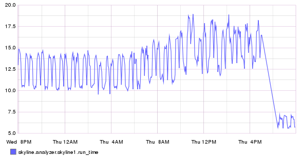
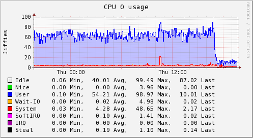
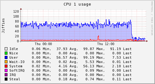
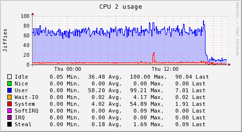
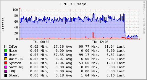
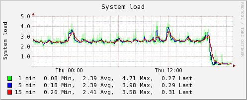
Optimizations results¶

These server graphs show the pre and post crucible update metrics related to CPU and loadavg for a dedicated Skyline server running on a 4 vCPU, 4GB RAM, SSD cloud server. The server is handling ~3000 metrics and is solely dedicated to running Skyline. It was upgraded from the Boundary branch version to Crucible.

It was running Analyzer, Mirage and Boundary, however these graphs clearly show the impact that the Analyzer optimizations have on the overall workload. Interestingly, after deployment the server is also running MySQL and the Panorama daemon in addition to what it was running before.

The server was running the skyline.analyzer.metrics branch Analyzer which was only a few steps away from Etsy master and those steps were related to Analyzer sending a few more Skyline metric namespaces to Graphite, in terms of Analyzer and the algorithms logic pre update were identical to Etsy master.